Updates
Renee's Update Page
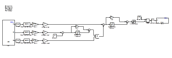
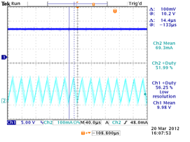
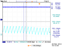
After building the PFC circuit we applied a 50% duty cycle from an open loop control and you can see in Figure 1 the current in channel 2 has a large ripple. With a PI controller the ripple will be reduced to create a clean current and a unity power factor. Channel 1 shows the output of the current sensor that inputs into the DSP.
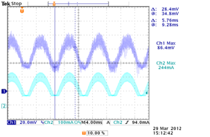
Open loop control, 50% duty cycle
Channel 1: output of current sensing circuitry and op amp input to the dsp
Channel 2: output of current probe (expected to be noisy because no PFC is implemented)
The 80mV out of the op amp can be converted by multiplying by the 1.25 voltage divider, then multiply by 50/4 for the current sensor, and divide by 5 to factor in the 5 loops around the current sensor gives you 250mV which the current probe is showing.
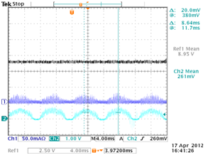
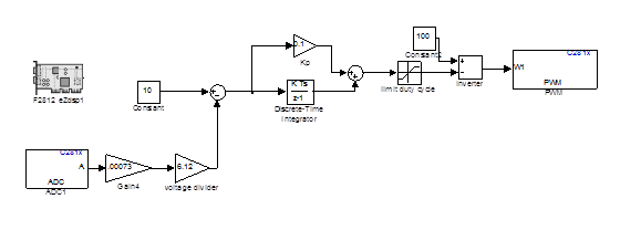
To test the hysteresis control of the current we applied the control you see in Figure 2. We simulated a current reference using a sine wave generator and an absolute value in simulink. After the actual current is read in through the ADC converter it is compared to the reference value and if the reference is greater the pwm is high and vice versa. The current that previously looked like channel 2 in figure 1 was smoothed out to the current that appears on channel 2 in figure 1
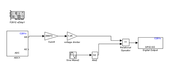
Simulink hysteresis control
Because the current being measured by the DSP is a rectified sign wave with an amplitude of approximately 80mV we simulated this in simulink as the reference current to match.
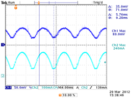
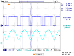
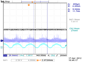
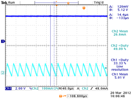
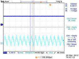
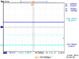
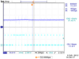
Figure 3 Figure 4
Channel 1: output of protection circuitry Channel : constantly adjusting PWM
Channel 2: current through inductor
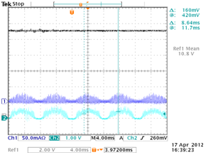
When testing the PFC controls the signal generator (XXXXX) used to create the sine wave would reach the current limit and lower the output voltage to an unusable value. In order to lower the current we increased the size of the load resistance to 10kW. This allowed the signal generator to output the full 10VpP sine wave, but this caused the circuit to go into discontinuous mode as seen in Figure 3 on channel 1. Even in discontinuous mode, the voltage could be controlled by changing the constant voltage reference in code composer when the control system in figure 5 was applied.
Simulink control system for PFC circut
As you can see in Figure 6 the output voltage of the PFC is very accurate when compared to the reference voltage entered.
 (A)
(A)
 (B)
(B)
 (C)
(C)
Figure 6
Channel 1 shows current through inductor, Channel 2 shows input voltage, and the Ref shows the output voltage. Reference values: (A) – 9, (B) – 7, (C) – 11.
Bi-directional Converter
Using the equation below we found the transfer function for our small scale buck converter to be: ![]()
clear all
close all
num = [29971 4.3e8];
den = [1 1.3587e3 1.4347e7]; % voltage mode control Fig-4-18
figure(1)
%f = linspace(30,30e3,500); % generate frequency points to be evaluated
f = logspace(1,4,500); % generate frequency points in log scale
w = 2*pi*f; % 'freqs' needs frequency in radians/sec
H = freqs(num, den, w) % to obtain frequency responses: amplitude and phase
amp = abs(H); % amp in linear scale
phase = angle(H)*180/pi;
magdB = 20*log10(amp); % magdB is the amplitude frequency response in decibel.
figure(1), subplot(211), semilogx(f, magdB(1,:)), title('amplitude response in dB'),grid
subplot(212),semilogx(f, phase(1,:)), title('phase response in degree')
grid, xlabel('frequency in Hz'),ylabel('degree')
Using the Matlab code in above we generated bode plots for the magnitude and phase of the power stage of the buck converter as seen in Figure 7
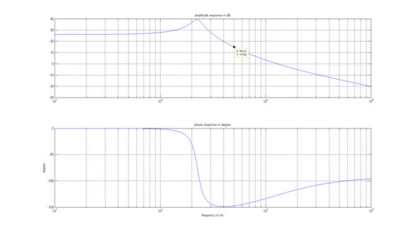
Phase and Magnitude plots for power stage
From Figure7 we can choose a crossover frequency. As ![]() we chose
we chose ![]() =500Hz. Therefore,
=500Hz. Therefore, ![]() or 5.7, and
or 5.7, and ![]() .
.
The transfer function of our PI control block is:
![]()
or
![]()
So the magnitude can be found by
and phase

In order to find the magnitude of the controller at our crossover frequency we use:
![]()
or
![]()
![]()
We set the phase margin to be:
![]()
We can then calculate the phase boost.
![]()
![]()
![]()
Once we have our phase boost we can calculate the phase of our controller at the crossover frequency
![]()
![]()
so using the earlier equations for the magnitude and phase of the controller you can find our gains to be:
![]()
Once we calculated our gains we applied them to a psim simulation seen in figure 8 to test the response of the controller
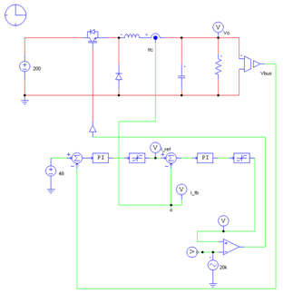
Figure 8
Psim model of control for the buck converter
You can see in figure 9 that the output voltage responded with little overshoot and a very fast settling time.
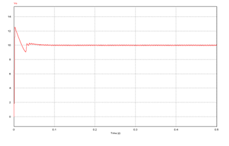
Figure 9
Output voltage response to psim simulation
We then built the simulink model seen in Figure 10 to run the control for the buck converter on the DSP. When the simuilnk file is compiled it generates a Ccode file in Code Composer and loads it onto the DSP. When testing with the small-scale model we had an input of 20V so we could expect the output to be smaller than that. The outputs were very accurate as seen in Figure 11
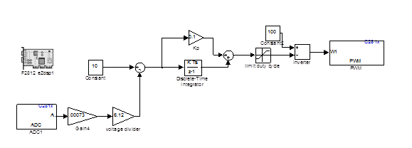 Figure 10
Simulink Control model used to generate C code for the buck converter
Channel 1 output shows the output voltage when the voltage reference is 10, 5,7 and 13.
We then used the same method described previously to calculate the Kp and Ki gains for the small-scale boost converter. After testing them in Psim we created the simulink model seen in Figure 12. This again was compiled into Code Composer to generate C code for the DSP to run.
Boost Converter control system in Simulink
With a 5V input into our system we can expect the output to be larger than that. As seen below in Figure 13 the output voltages matched the constant reference value accurately.


Results from closed loop boost converter. Channel 1 shows output voltage.