![]()
![]()
![]()
![]()
![]()
Image Generator to Support the Application of a Haptic
Device for the Simulation of Arthroscopic Surgery
By
Renata Zabawa
Project Advisor:
Dr. Thomas L. Stewart
Submission Date: May 8, 2006
EE451 Senior Capstone Project
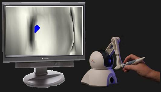
Magnetic Resonance Imaging (MRI) creates hundreds of images that each shows a cross section of the knee. The goal of this project is to take the cross sections of a knee MRI and extract a three dimensional model of the cartilage. This model is used to simulate a surgeon’s view during arthroscopic surgery. A second goal is to apply these results to simulate the arthroscopic surgery with a haptic feedback system. The simulations will aide medical students by allowing them to practice arthroscopic surgery in a simulator before actually performing a real arthroscopic surgery.
This project will take the data of each MRI scan and create a data matrices that can be used to create a three dimensional model of the cartilage in the knee. An example of an MRI scan is seen in Figure 1. The cartilage data is then split into its two menisci. Light and view are used to simulate the surgeon’s view during arthroscopic surgery. This image could eventually be used with a haptic feedback system to simulate an arthroscopic surgery. The haptic device allows one to feel the image as it is viewed. This would allow medical students to practice arthroscopic knee surgery before performing it on an actual person. This project manipulates and smoothes the data, so this is not a diagnostic device. It is a training tool.
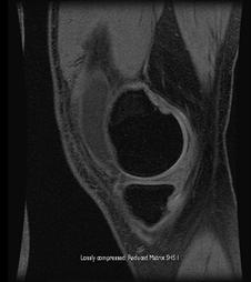
Figure1: MRI Scan of Knee
Figure 2 shows the overall system block diagram. The input is the image data from the MRI scans. The MRI scans will be 500 X 500 pixels each. Each cross section of the knee is stacked together and this data is used to create the model of the cartilage and generate the simulation of the arthroscopic surgery.
Figure 2: Overall System Block Diagram
Figure 3 shows a high-level block diagram for the entire system. The MRI scan data points each show a cross sections of the knee as seen in Figure 1. An image processing block uses Matlab to generate a 3-D model of the cartilage. Then the model is used to create a simulation of an arthroscopic surgery.
Figure 3: High Level Block Diagram
Figure 4 illustrates the software used to create the original cartilage model. Matlab loads the data from an MRI scan. To generate the three dimensional model of the cartilage, a few steps must be taken. First, the MRI data is loaded into Matlab. Then isosurfaces and isocaps are used on each set of MRI data points. Isosurfaces use the data to create a three-dimensional analog. It computes the surface faces and vertices from the 3-D volume of data. The surfaces and vertices are connected to form the overall structure of the meniscus. An isosurface has a specified iso-level. The volume inside, which is set to a color specified in the program, contains values greater than the isovalue. The volume outside contains values less than the isovalue.
Isocaps use raw data to reveal details of the interior of the isosurfaces. They show a cross-sectional view of the interior of the cartilage. For this project, the overall structure of the meniscus is what is being utilized. The renderer to display the cartilage model is set to zbuffers. Zbuffers is the only renderer in Matlab that allows phong lighting. Phong lighting is used because it works best with curves. It produces a degree of realism in three-dimensional objects by considering the three elements - diffuse, specular and ambient for each point on a surface.

Figure4: Image Processing Block Diagram
The model created is seen in Figure 5. It shows the model created using the raw data with the tear. The thickness of the cartilage from the MRI scans is about 0.1 inches. The model created in Matlab blows up the size of the cartilage on the screen. This is done with slices of data that are taken to view the 0.1 inch thick cartilage. To do this, the model must stretch the data. There are not enough points of data which cause the image created to appear uneven. This is not acceptable for the project, so the data must be smoothed before the surgeon’s view of it can be created. The code to create the cartilage model seen in Figure 5 is found in Appendix A.
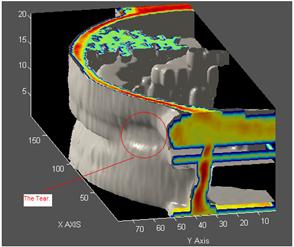
Figure5: Original Model of Cartilage
Figure 6: Graphics Block Diagram
Figure 6 shows the graphics that will be accomplished with Matlab. Once a 3-D image of the cartilage is created and the menisci are split, the image must be smoothed. To smooth the image, it must first be visually inspected. The tear is picked out and the data points where the tear exists are separated from the complete cartilage model. The complete cartilage model and tear are smoothed separately each by a 7x7x7 averaging filter. Then the tear data is put back into the complete model in its original location. The overall model is smoothed with a 3x3x3 averaging filter. This allows the model to be viewed with light at a close proximity without ripples and distortion.
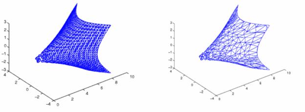
To create the model, the isosurfaces generate vertices and faces that are filled in by patches. Fewer patches in an image cause it to appear smoother. Matlab will reduce the number of patches while preserving the shape of the overall image. An example of a structure of faces and vertices created by patches is shown in Figure 7. The patches of this object are reduced by 15% and the structure is now seen in Figure 8. In this program half of the patches are eliminated, which decreases the amount of surface ripples and shadows created when light is added to the model.
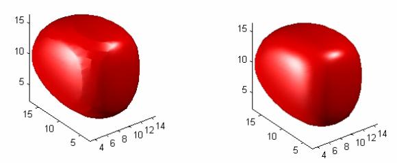
The surface normals greatly affect the visual appearance of lit isosurfaces. Surface normals are three dimensional vectors that are perpendicular to the plane. A triangle’s surface normal is calculated as the vector cross product of two edges of the triangle. Many times, the triangles used to draw the isosurface define the normals, which are called triangle normals. A lit sphere with triangle normals is seen in Figure 9. In this case, each triangle is lit identically. Each triangle’s flatness is obvious to the eye. Matlab has an isonormals function, which uses the volume data to calculate the vertex normals. This is called data normals and they are seen on a lit sphere in Figure 10. Each vertex of a triangle is lit individually, which causes a smoother appearance. This is most significantly seen in curved surfaces. For the application of this program, data normals are used to light surfaces. The code to create the smoothed cartilage model is seen in Appendix B.
The properties of light are set individually for the isosurfaces and isocaps. They can be set when the patches are defined or after the patches have been created. This program sets the properties at the time the patches are created. The patch has a property that sets the face color of the image. This sets the color of the patch in [R, G, B]. The cartilage model was given a red value of 255/256, a green value of 255/256 and a blue value of 240/256. This gives the model an ivory color.
The ambient strength controls the intensity of the ambient component of the light reflected from the object. This controls the amount of light that gets added to a scene no matter what. In this project the ambient strength is set to zero. This setting allows no light, so the areas of the patch without light are not lit.
Face lighting is set to phong. The effect of light is determined by interpolating the vertex normals across the faces and calculating each pixels reflectance. It is best to view curved surfaces with this option.
The specular exponent controls the size of the specular spot. It controls the size of the area lit up. It can be set from 1 to 500. It is set to two, which is one of the largest highlighted areas possible.
The specular strength determines the intensity of the specular component of the light reflected from the object, which means the higher the specular component, the more mirror-like the object appears. The mirror-like model makes it easier to see the indentations of the tear. Specular light is the light that gets reflected into a particular direction. The specular strength can be set from 0 to 1 at the highest. For this project 1 was chosen to allow ease in seeing the tear.
The diffuse strength determines the intensity of the diffuse component of the light reflected from the object. It is the light that hits a surface and gets scattered equally into all directions. It is used with ambient strength to darken or lighten the background where the light isn’t directly hitting. This is also set to 0. For this project, the light that hits the model should not reflect onto other parts of the model.
The specular color reflectance controls the color of the specularly reflected light. The project needs the light reflected to be determined by the model. To have it depend on both the color of the object from which it reflects and the color of the light source the property is set to 0. Code to create a pyramid to be used as a tutorial with the light properties and light position is seen in Appendix H.
To simulate the arthroscopic surgeon’s view, three properties must be controlled. They are the camera position and target and the light position. The camera target can be set to anywhere on the figure. It will point to the camera target, which can also point to any space in the figure. The light position is also set to anywhere on the figure. The light can either come from the position it is set to or just from that direction. If the light comes from the position it is set at, it behaves much like a spotlight. When light just comes from a direction it behaves similar to the sun. The light color is set to white so the color of the cartilage is seen. A tutorial for view and the camera functions was also created in Matlab. It creates a multicolored pyramid, so the view can be manipulated to look at sides of different colors. The code to create the pyramid is in Appendix I.
Matlab functions are used to put the light on the meniscus model and to view it from different positions. These functions create an image on the computer monitor that simulates a surgeon’s view during arthroscopic surgery. The code to set the view and light position is included in Appendix C. Code to set the view and light position and then zoom in on the tear is seen in Appendix D. An m-file was also created to leave the light position stationary, but vary the view as a surgeon might do. This is included in Appendix G. Figure 11 exemplifies the actual view a surgeon sees. It illustrates torn menisci.
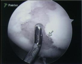
Figure 11: Arthroscopic Surgery View of Torn Cartilage
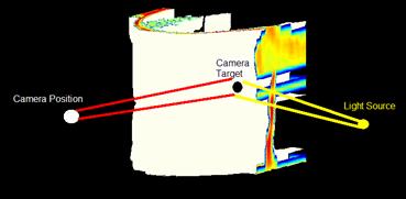
Figure 12: Model of Single Meniscus with Light and View
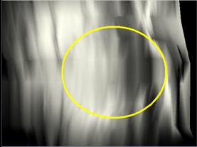
Figure 13: Raw Model
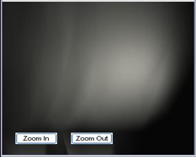
Figure 14: Matlab View of Healthy Cartilage
Figure 5: Matlab View of Torn Cartilage
The model of a single meniscus using the techniques discussed above was created and the light and view were set as they would be in an arthroscopic surgery. The setup is seen in Figure 12. The tear of the raw cartilage model was first looked at and is seen in Figure 13. The surgeon’s view shows ripples and distortion, which interfere with the view of the tear. The area circled is where the tear in the cartilage is located.
After the data has been smoothed and manipulated to create the final model, light and the view were again put on the model. First, the light and view were set to look at healthy cartilage. The output of the view was as expected and is seen in Figure 14. Then the light and view were moved to the tear in the cartilage as seen in Figure 15. The actual tear of the cartilage has been distorted. This is due to the smoothing filters that were applied to the cartilage model. Since the model is not used for diagnostic purposes and is made for the purpose of training the changes to the cartilage model are insignificant. The model of the tear seen in Figure 16 resembles the actual tear, which is seen in Figure 11. The tear is easily visible and the view is the same as that of an arthroscopic surgery.
The cartilage model with the proper lighting and view generated a simulation of the arthroscopic surgeon’s view. The goal of this project was met. This project proves that by using the proper light and view on a model created from MRI data the view of an arthroscopic surgery can be generated. The work done in Matlab and some preliminary work done in C++ with the haptic feedback device suggests that the same view of the arthroscopic surgery can be displayed and felt with the haptic device. The code to create Matlab data that the haptic dvice can use is seen in Appendix E. Appendix F describes what needs to be done with the data Matlab will generate.
From Matlab data, an image can be created and felt with the haptic device. By setting the light and view in OpenGL similar to the setting used in Matlab, the view would simulate that of an arthroscopic surgeon. The feel of the image created can also be simulated using OpenGL. A test cube has been created in C++ and the code is seen in Appendix J. A thorough description of how to run the code is found in Appendix K. This allows one to move the view that was created in this project and also feel the cube. Trying to implement the arthroscopic surgeon’s view with the haptic feedback device would be excellent future work on this project. It could be used in the future as a training device for medical students in arthroscopic knee surgeries.
No patents have been made for the simulation of an arthroscopic knee surgery. Similar patents have been obtained. One patent was issued to Kurt Amplatz for a medical simulator that enables demonstration, trial and test of insertion of torqueable elongated members, such as guide wires or catheters, into small body passages. Another patent was issued to Nobuhiko Mukai, Masayuki Harada and Katsunobu Muroi for a simulated medical treatment virtually executed by an operator with a simulated medical instrument, while using the virtual model information. Wendy Plesniak, Ravikanth Pappu and Stephen Benton received a patent for a coincident visuo-haptic workspace, which allows a user to see, feel, and interact with synthetic objects. There is a spatial display that enables synthetic objects to become a part of the user's manipulatory space.
Hill, F.S. Jr. (1990). Computer Graphics using OpenGL, Second Edition. New Jersey, Upper
Saddle River: Prentice Hall.
Holland, Thomas & Marchand, Patrick (2003). Graphics and GUIS with Matlab, Third Edition.
Washington, DC: Chapman & Hall/CRC.
Links, Jonathan and Prince, Jerry. Medical Imaging: Signals and Systems. New Jersey: Pearson Education, 2006.
Matlab, Version 7.0.1, The MathWorks Inc., Natrick, MA 01760, 2004.
Location: Desktop\Testing\MATLABfiles\gen3d_femur_knee1
%generate original model to find tear
clc
clear
load('seg_img_femur_knee1','-mat');
newcut=squeeze(cimg6);
Ds = smooth3(newcut);
figure,
whitebg('k')
hiso = patch(isosurface(Ds,6),...
'FaceColor',[253/256 245/256 230/256],...
'EdgeColor','none');
hcap = patch(isocaps(newcut,6),...
'FaceColor','interp',...
'EdgeColor','none');
colormap;
view(45,30)
axis tight
daspect([1,1,.4])
lightangle(145,30); lighting phong
isonormals(Ds,hiso);
set(hcap,'AmbientStrength',.6)
set(hiso,'SpecularColorReflectance',0,'SpecularExponent',50)
Location: Desktop\Testing\MATLABfiles\checkfemur3d
clc
clear
% load data from the file seg_img_femur_knee1 and delete all info not
% needed
load('seg_img_femur_knee1','-mat');
clear cimg4
clear cimg5
newcut=(cimg6);
%Smooth data as explained in paper
y=smooth3(newcut);
Ds = smooth3(newcut,'box',[7 7 7]);
Ds(51:62,20:40,12:15)=y(51:62,20:40,12:15);
Ds=smooth3(Ds);
%Create new figure with black background for model to be displayed
figure,
whitebg('k')
%Isosurfaces drawn using smoothed Ds data from Ds. Patches created for
%faces and vertices of isosurfaces
hiso = patch(isosurface(Ds,6),...
'FaceColor',[255/256 255/256 240/256],...%ivory
'EdgeColor','none',... %peachier 253/256 245/256 230/256
'AmbientStrength',0,...
'faceLighting','phong',...
'SpecularExponent',2,...
'SpecularStrength',1,...
'BackfaceLighting','unlit',...
'DiffuseStrength',0,...
'SpecularColorReflectance',0);
%Isocaps drawn with raw data
hcap = patch(isocaps(Ds,6),...
'FaceColor','interp',...
'EdgeColor','none',...
'AmbientStrength',0,...
'faceLighting','phong',...
'SpecularExponent',2,...
'SpecularStrength',.5,...
'BackfaceLighting','unlit',...
'DiffuseStrength',0,...
'SpecularColorReflectance',0);
%Reducepatch- reduces the number of faces in patch and preserve the overall
%shape of the patch
reducepatch(hiso, .5)
lighting phong
%Isonormals – Produces smoother appearing isosurfaces.
isonormals(Ds,hiso);
colormap;
view(45,30)
axis tight
%Set renderer of figure to zbuffers, allows phong lighting (can’t do in
%opengl).
set(gcf,'Renderer','zbuffer')
xlabel('x-axis')
ylabel('y-axis')
zlabel('z-axis')
Location: Desktop\Testing\MATLABfiles\viewtear
%Set the position and properties of light
light('Position',[20 70 14],'Style','local','Color','w')
%Set camera position and camera target
camtarget([14 15 14])
campos([5,70,14])
Location: Desktop\Testing\MATLABfiles\zoomtear
%Set the position and properties of light
light('Position',[15 60 14],'Style','local','Color','w')
%Set camera position and camera target
camtarget([14 15 14])
campos([5,70,14])
%Zoom in on tear
zoom(8)
Location: Desktop\Testing\MATLABfiles\getData
% get faces and vertices for haptic device
pf=get(hiso,'faces') ;
pv=get(hiso,'vertices');
[r,c]=size(pf);
for i=1:r
for j=1:3
pf(i,j)=pf(i,j)-1;
end
end
pf1=get(hcap,'faces') ;
pv1=get(hcap,'vertices');
[r1,c1]=size(pf1);
for i=1:r1
for j=1:3
pf1(i,j)=pf1(i,j)-1;
end
end
The haptic feedback system uses .dat files that contain the vertices and faces of the object it will create. The .dat files are created using Matlab data. Once the data has been compiled in Matlab with the code seen in Appendix D, then each variable must be copied and pasted into a text file. The file should be saved as a .dat file with the name that is called by the haptic feedback system. The files created must be put into the same folder as the .cpp file that calls the .dat files.
Location: Desktop\Testing\MATLABfiles\move_tear
%save the model and open it
saveas(gcf,'MyModel','m')
MyModel
%change the view while keeping the light at the same position
n=0.2; %how long to pause for
pos=get(gca,'CameraPosition');
for dx=-.5:.05:.75
pause(n)
camdolly(dx,0,0)
drawnow
end
for dx=-.55:.05:0
pause(n)
camdolly(dx,0,0)
drawnow
end
for dy=-.25:.05:.5
pause(n)
camdolly(0,dy,0)
drawnow
end
for dy=-.4:.05:0
pause(n)
camdolly(0,dy,0)
drawnow
end
%delete 'LK.fig'
%delete 'LK.m'
Appendix H:
Location: Desktop\Testing\MATLABfiles\TestLight
%Create pyramid to test light with
%Generate [M x N x O] matrix of Data
figure;
for z=1:1:101 % Generates a [M x N x O] matrix of white
for y=1:1:101
for x=1:1:101
pic(x,y,z)=250;
end
end
end
r=0; %set radius
for z=1:1:101
r=r+1;
for y=1:1:101
for x=1:1:101
if(r>=4 && r<=50) %if the radius is between a ceratin value create a circle
circle=x^2+y^2-r^2; %use x^2+y^2-r^2 to determine of the point lies in on or outside the circle
if(circle<=0) %if circle is 0 point lies on the circle and if < 0 it lies in the circle
%this function generates the fourth quadrant of a circle (1/4 of it)- makes circle black
y1=y+50; %shift the circle to the middle of the plot - this y for the 3rd and 4th quadrant
x1=x+50; %shift circle to middle- this x for 1st and 2nd quadrant
y2=50-(y-1); %y for 1st and second quadrant
x2=50-(x-1); %x for 2nd and 3rd qudrant
pic(x1,y1,z)=0; %4th quadrant of circle (1/4)
pic(x2,y1,z)=0; %3rd quadrant of circle (1/4)
pic(x1,y2,z)=0; %1st quadrant of circle (1/4)
pic(x2,y2,z)=0; %2nd quadrant of circle (1/4)
end
end
end
end
end
%The [M x N x O] Matrix has been created
%Now we will display it in 3-D
pic2=squeeze(pic);
dpic=smooth3(pic2);
hiso = patch(isosurface(dpic,6),...
'FaceColor',[.7 .6 1],...
'EdgeColor','none',...
'SpecularExponent',1,...
'AmbientStrength',0);
colormap;
view(3)
axis tight
Location: Desktop\Testing\MATLABfiles\makePyramid
%Create Pyramid to practice camera view
figure(1);
vertex=[-5 -5 0; %vertex 1
5 -5 0; %vertex 2
5 5 0; %vertex 3
-5 5 0; %vertex 4
0 0 -10;]; %vertex 5
%for quadrilateral faces and triangular faces, max # rows is 4
%only 3 vertices for trianles so put NaN in fourth column
faces=[1 2 3 4; %Face F1
1 2 5 NaN; %Face F2
2 3 5 NaN; %Face F3
3 4 5 NaN; %Face F4
4 1 5 NaN]; %Face F5
p=patch('vertices',vertex,...
'faces',faces,...
'FaceVertexCData',hsv(5),...
'FaceColor','flat');
axis([-8 10 -10 9 -10 0]);
view(3);
This file creates a cube in C++ with the haptic device.
Location: Desktop\Testing\cube_hap.cpp
#include <math.h>
#include <assert.h>
#ifdef WIN32
#include <windows.h>
#endif
#include <C:\Documents and Settings\dgaddipa\Desktop\New Folder\GL/gl.h>
#include <C:\Documents and Settings\dgaddipa\Desktop\New Folder\3DTouch\utilities\include\GL/glut.h>
#include <C:\Documents and Settings\dgaddipa\Desktop\New Folder\3DTouch\include\HL/hl1.h>
#include <C:\Documents and Settings\dgaddipa\Desktop\New Folder\3DTouch\utilities\include\HDU/hduMatrix1.h>
#include <C:\Documents and Settings\dgaddipa\Desktop\New Folder\3DTouch\utilities\include\HDU/hduError1.h>
#include <C:\Documents and Settings\dgaddipa\Desktop\New Folder\3DTouch\utilities\include\HLU/hlu1.h>
typedef GLfloat point3[3];
typedef GLfloat color [4];
#define CURSOR_SIZE_PIXELS 20
static HHD hHD = HD_INVALID_HANDLE;
static HHLRC hHLRC = 0;
// shape id for shape we will render haptically
HLuint cubeShapeId;
HLuint cubeShapeId1;
static double gCursorScale;
static GLuint gCursorDisplayList = 0;
/* Function prototypes. */
void glutDisplay(void);
void glutReshape(int width, int height);
void glutIdle(void);
void exitHandler(void);
void initGL();
void initHL();
void initScene();
void drawSceneHaptics();
void drawSceneGraphics();
void drawCursor();
void updateWorkspace();
/****************************************************************************
Initializes GLUT for displaying a simple haptic scene
****************************************************************************/
int main(int argc, char *argv[])
{
glutInit(&argc, argv);
glutInitDisplayMode(GLUT_DOUBLE | GLUT_RGB | GLUT_DEPTH);
glutInitWindowSize(500, 500);
glutCreateWindow("Cube Example");
/* Set glut callback functions. */
glutDisplayFunc(glutDisplay);
glutReshapeFunc(glutReshape);
glutIdleFunc(glutIdle);
/* Provide a cleanup routine for handling application exit. */
atexit(exitHandler);
initScene();
glutMainLoop();
return 0;
}
/****************************************************************************
GLUT callback for redrawing the view
****************************************************************************/
void glutDisplay()
{
drawSceneHaptics();
drawSceneGraphics();
glutSwapBuffers();
}
/****************************************************************************
GLUT callback for reshaping the window. This is the main place where the
viewing and workspace transforms get initialized.
****************************************************************************/
void glutReshape(int width, int height)
{
static const double kPI = 3.1415926535897932384626433832795;
static const double kFovY = 40;
double nearDist, farDist, aspect;
glViewport(0, 0, width, height);
/* Compute the viewing parameters based on a fixed fov and viewing
* a canonical box centered at the origin
*nearDist and farDist are in radians respectively 2.8,4.8*/
nearDist = -10.0;//(1.0 / tan((kFovY / 2.0) * kPI / 180.0));
farDist = 10;//nearDist + 2.0;
aspect = (double) width / height;
glMatrixMode(GL_PROJECTION);
glLoadIdentity();
//gluPerspective(kFovY, aspect, nearDist, farDist);
glOrtho(-5,5,-5,5,5,20);
/* Place the camera down the Z axis looking at the origin */
glMatrixMode(GL_MODELVIEW);
glLoadIdentity();
gluLookAt(-6, 6, 6,
-.25, .25, .25,
0, +1, 0);
updateWorkspace();
}
/***************************************************************************
GLUT callback for idle state. Use this as an opportunity to request a redraw.
Also check for HLAPI errors that have occurred since the last idle check
****************************************************************************/
void glutIdle()
{
HLerror error;
while (HL_ERROR(error = hlGetError()))
{
fprintf(stderr, "HL Error: %s\n", error.errorCode);
if (error.errorCode == HL_DEVICE_ERROR)
{
hduPrintError(stderr, &error.errorInfo,
"Error during haptic rendering\n");
}
}
glutPostRedisplay();
}
/*****************************************************************************
Initialize the scene. Handle initializing both OpenGL and HL
****************************************************************************/
void initScene()
{
initGL();
initHL();
}
/****************************************************************************
Setup general OpenGL rendering properties, like lights, depth buffering, etc.
****************************************************************************/
void initGL()
{
static const GLfloat light_model_ambient[] = {1.0f, 1.0f, 1.0f, 1.0f};
static const GLfloat light0_diffuse[] = {1.0f, 1.0f, 1.0f, 1.0f};
static const GLfloat light0_direction[] = {0.0f, 0.0f, 5.0f, 0.0f};
/* Enable depth buffering for hidden surface removal. */
glDepthFunc(GL_LEQUAL);
glEnable(GL_DEPTH_TEST);
/* Cull back faces. */
glCullFace(GL_BACK);
glEnable(GL_CULL_FACE);
/* Set lighting parameters */
glEnable(GL_LIGHTING);
glEnable(GL_NORMALIZE);
glShadeModel(GL_SMOOTH);
glLightModeli(GL_LIGHT_MODEL_LOCAL_VIEWER, GL_TRUE);
glLightModeli(GL_LIGHT_MODEL_TWO_SIDE, GL_TRUE);
glLightModelfv(GL_LIGHT_MODEL_AMBIENT, light_model_ambient);
glLightfv(GL_LIGHT0, GL_DIFFUSE, light0_diffuse);
glLightfv(GL_LIGHT0, GL_POSITION, light0_direction);
glEnable(GL_LIGHT0);
}
/****************************************************************************
Initialize the HDAPI. This involves initing a device configuration, enabling
forces, and scheduling a haptic thread callback for servicing the device.
****************************************************************************/
void initHL()
{
HDErrorInfo error;
hHD = hdInitDevice(HD_DEFAULT_DEVICE);
if (HD_DEVICE_ERROR(error = hdGetError()))
{
hduPrintError(stderr, &error, "Failed to initialize haptic device");
fprintf(stderr, "Press any key to exit");
getchar();
exit(-1);
}
hHLRC = hlCreateContext(hHD);
hlMakeCurrent(hHLRC);
// Enable optimization of the viewing parameters when rendering
// geometry for OpenHaptics
hlEnable(HL_HAPTIC_CAMERA_VIEW);
// generate id's for the three shapes
cubeShapeId = hlGenShapes(1);
cubeShapeId1 = hlGenShapes(1);
hlTouchableFace(HL_FRONT);
}
/****************************************************************************
This handler will get called when the application is exiting.
Deallocates any state and cleans up.
****************************************************************************/
void exitHandler()
{
// deallocate the sphere shape id we reserved in in initHL
hlDeleteShapes(cubeShapeId, 1);
hlDeleteShapes(cubeShapeId1, 1);
// free up the haptic rendering context
hlMakeCurrent(NULL);
if (hHLRC != NULL)
{
hlDeleteContext(hHLRC);
}
// free up the haptic device
if (hHD != HD_INVALID_HANDLE)
{
hdDisableDevice(hHD);
}
}
/****************************************************************************
Use the current OpenGL viewing transforms to initialize a transform for the
haptic device workspace so that it's properly mapped to world coordinates.
****************************************************************************/
void updateWorkspace()
{
GLdouble modelview[16];
GLdouble projection[16];
GLint viewport[4];
glGetDoublev(GL_MODELVIEW_MATRIX, modelview);
glGetDoublev(GL_PROJECTION_MATRIX, projection);
glGetIntegerv(GL_VIEWPORT, viewport);
hlMatrixMode(HL_TOUCHWORKSPACE);
hlLoadIdentity();
/* fit haptic workspace to view volume */
hluFitWorkspace(projection);
/* compute cursor scale */
gCursorScale = hluScreenToModelScale(modelview, projection, viewport);
gCursorScale *= CURSOR_SIZE_PIXELS;
}
void drawCube()
{
glPushMatrix();
glRotatef(30,1,1,0);
glEnable(GL_COLOR_MATERIAL);
point3 vertices[8]={{-1.0f, -1.0f, -1.0f},
{-1.0f, -1.0f, 1.0f},
{-1.0f, 1.0f, -1.0f},
{-1.0f, 1.0f, 1.0f},
{ 1.0f, -1.0f, -1.0f},
{ 1.0f, -1.0f, 1.0f},
{ 1.0f, 1.0f, -1.0f},
{ 1.0f, 1.0f, 1.0f} };
GLfloat white[]={1.0, 1.0, 1.0, 1.0};
glMaterialfv(GL_FRONT_AND_BACK, GL_AMBIENT, white );
glMaterialfv(GL_FRONT_AND_BACK, GL_DIFFUSE, white );
glEnable(GL_COLOR_MATERIAL);
glBegin(GL_QUADS);
//make the front quadrant RED
glColor3f(1.0, 0.0, 0.0);
hlMaterialf(HL_FRONT_AND_BACK, HL_STIFFNESS, .001f);
hlMaterialf(HL_FRONT_AND_BACK, HL_DAMPING, .0001f);
hlMaterialf(HL_FRONT_AND_BACK, HL_STATIC_FRICTION, .0001f);
hlMaterialf(HL_FRONT_AND_BACK, HL_DYNAMIC_FRICTION, .0001f);
glVertex3fv(vertices[1]);
glVertex3fv(vertices[5]);
glVertex3fv(vertices[7]);
glVertex3fv(vertices[3]);
//make the top of the square GREEN
glColor3f(0.0, 1.0,0.0);
hlMaterialf(HL_FRONT_AND_BACK, HL_STIFFNESS, .2f);
hlMaterialf(HL_FRONT_AND_BACK, HL_DAMPING, 0.1f);
hlMaterialf(HL_FRONT_AND_BACK, HL_STATIC_FRICTION, 0.01f);
hlMaterialf(HL_FRONT_AND_BACK, HL_DYNAMIC_FRICTION, 0.01f);
glVertex3fv(vertices[7]);
glVertex3fv(vertices[6]);
glVertex3fv(vertices[2]);
glVertex3fv(vertices[3]);
//Make the back quadrant BLUE
glColor3f(0.0, 0.0,1.0);
hlMaterialf(HL_FRONT_AND_BACK, HL_STIFFNESS, .99f);
hlMaterialf(HL_FRONT_AND_BACK, HL_DAMPING, 0.1f);
hlMaterialf(HL_FRONT_AND_BACK, HL_STATIC_FRICTION, 0.2f);
hlMaterialf(HL_FRONT_AND_BACK, HL_DYNAMIC_FRICTION, 0.3f);
glVertex3fv(vertices[2]);
glVertex3fv(vertices[6]);
glVertex3fv(vertices[4]);
glVertex3fv(vertices[0]);
//Make the right quadrant PURPLE/PINK
glColor3f(1.0, 0.0,1.0);
hlMaterialf(HL_FRONT_AND_BACK, HL_STIFFNESS, .0001f);
hlMaterialf(HL_FRONT_AND_BACK, HL_DAMPING, 0.1f);
hlMaterialf(HL_FRONT_AND_BACK, HL_STATIC_FRICTION, 0.01f);
hlMaterialf(HL_FRONT_AND_BACK, HL_DYNAMIC_FRICTION, 0.01f);
glVertex3fv(vertices[5]);
glVertex3fv(vertices[4]);
glVertex3fv(vertices[6]);
glVertex3fv(vertices[7]);
//make the bottom of the square ORANGE
glColor3f(1.0, 0.4,0.0);
hlMaterialf(HL_FRONT_AND_BACK, HL_STIFFNESS, .99f);
hlMaterialf(HL_FRONT_AND_BACK, HL_DAMPING, 0.1f);
hlMaterialf(HL_FRONT_AND_BACK, HL_STATIC_FRICTION, 0.2f);
hlMaterialf(HL_FRONT_AND_BACK, HL_DYNAMIC_FRICTION, 0.3f);
glVertex3fv(vertices[4]);
glVertex3fv(vertices[5]);
glVertex3fv(vertices[1]);
glVertex3fv(vertices[0]);
//make the left quadrant YELLOW
glColor3f(1.0, 1.0,0.0);
hlMaterialf(HL_FRONT_AND_BACK, HL_STIFFNESS, .2f);
hlMaterialf(HL_FRONT_AND_BACK, HL_DAMPING, 0.1f);
hlMaterialf(HL_FRONT_AND_BACK, HL_STATIC_FRICTION, 0.01f);
hlMaterialf(HL_FRONT_AND_BACK, HL_DYNAMIC_FRICTION, 0.01f);
glVertex3fv(vertices[0]);
glVertex3fv(vertices[1]);
glVertex3fv(vertices[3]);
glVertex3fv(vertices[2]);
glEnd();
glPopMatrix();
glPopAttrib();
}
/****************************************************************************
The main routine for displaying the scene. Get the latest snapshot of state
from the haptic thread and use it for displaying a 3D cursor.
****************************************************************************/
void drawSceneGraphics()
{
glClear(GL_COLOR_BUFFER_BIT | GL_DEPTH_BUFFER_BIT);
// draw 3D cursor at haptic device position
drawCursor();
drawCube();
}
/****************************************************************************
The main routine for rendering scene haptics.
Renders the sphere haptically.
****************************************************************************/
void drawSceneHaptics()
{
// start haptic frame - must do this before rendering any haptic shapes
hlBeginFrame();
// set material properties for the shapes to be drawn
// start a new haptic shape, use the feedback buffer to
// capture OpenGL geometry for haptic rendering
hlBeginShape(HL_SHAPE_FEEDBACK_BUFFER, cubeShapeId);
hlTouchableFace(HL_FRONT);
drawCube();
hlEndShape();
hlEndFrame();
}
/****************************************************************************
Draw a 3D cursor for the haptic device using the current local transform,
the workspace to world transform and the screen coordinate scale.
****************************************************************************/
void drawCursor()
{
static const double kCursorRadius = 0.5;
static const double kCursorHeight = 1.5;
static const int kCursorTess = 15;
HLdouble proxyxform[16];
GLUquadricObj *qobj = 0;
glPushAttrib(GL_CURRENT_BIT | GL_ENABLE_BIT | GL_LIGHTING_BIT);
glPushMatrix();
if (!gCursorDisplayList)
{
gCursorDisplayList = glGenLists(1);
glNewList(gCursorDisplayList, GL_COMPILE);
qobj = gluNewQuadric();
gluCylinder(qobj, 0.0, kCursorRadius, kCursorHeight,
kCursorTess, kCursorTess);
glTranslated(0.0, 0.0, kCursorHeight);
gluCylinder(qobj, kCursorRadius, 0.0, kCursorHeight / 5.0,
kCursorTess, kCursorTess);
gluDeleteQuadric(qobj);
glEndList();
}
/* Get the proxy transform in world coordinates */
hlGetDoublev(HL_PROXY_TRANSFORM, proxyxform);
glMultMatrixd(proxyxform);
/* Apply the local cursor scale factor. */
glScaled(gCursorScale, gCursorScale, gCursorScale);
glEnable(GL_COLOR_MATERIAL);
glColor3f(1.0, 1.0, 1.0);
glCallList(gCursorDisplayList);
glPopMatrix();
glPopAttrib();
}
This explains how to run the file in Appendix J.
Build the project.
Project-Settings
Select the C/C++ Tab
Change:
Category: Code Generation
Use run-time Library: Multithreaded DLL
Open Desktop\Testing\Library.txt
Select All, Copy the information
Select the Link Tab
Paste all data copied to the end of the Object/library Modules
Hit OK.
Compile, Build, Execute.